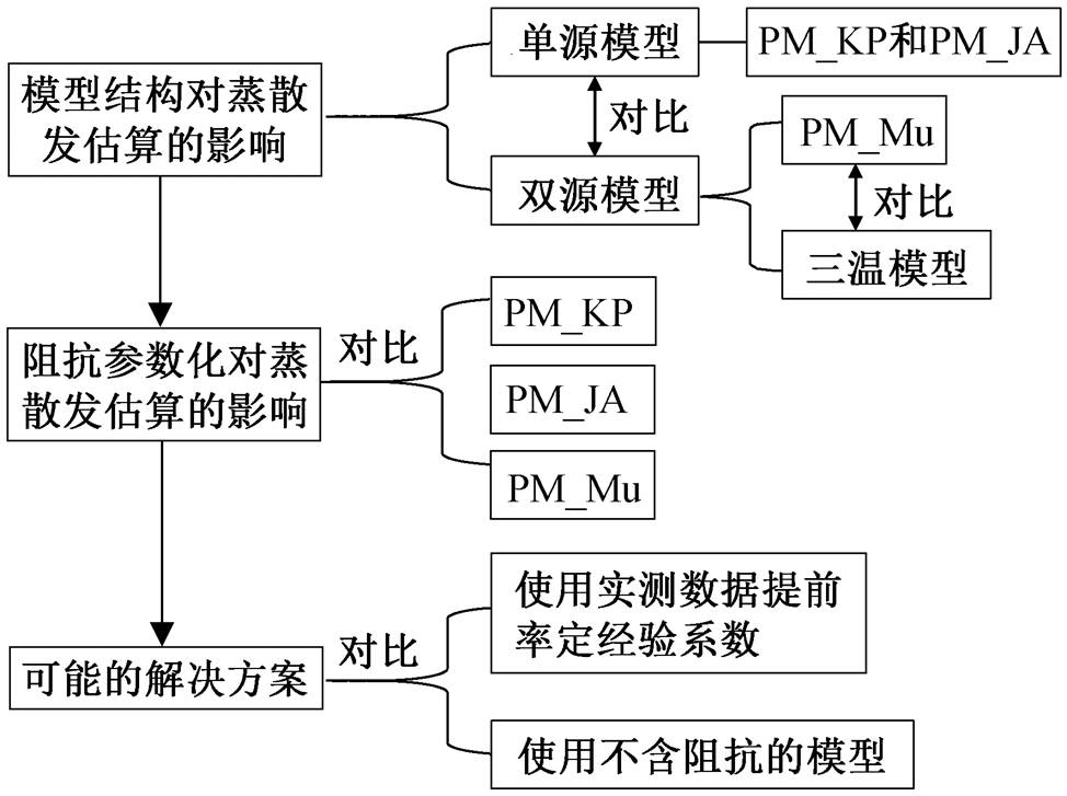
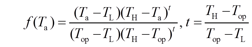
图1 研究框架示意图
Fig. 1 A schematic of the workflow
摘要 基于 2012 年黑河绿洲 HiWATER 高密度通量观测数据, 对比研究模型结构差异(单源 Penman-Monteith/ PM 公式与双源 PM 公式、双源 PM 公式与双源三温模型)以及 PM 公式中阻抗参数化差异对蒸散发估算的影响。结果表明: 1)与模型结构相对复杂的双源 PM 公式相比, 单源 PM 公式计算的蒸散发平均相对误差(MAPE)为 34%, 略优于双源 PM 公式的 40%; 2)对于两种模型结构差异显著的双源模型, 模型中不含阻抗参数的三温模型比模型中含阻抗参数的 PM 公式具有更高的估算精度, 前者的 MAPE 为 18% (R2=0.85), 后者为40% (R2=0.34); 3)两种单源和一种双源阻抗参数化方法导致 PM 公式计算的蒸散发出现不同程度的差异, MAPE 可相差 6%; 4)使用先验知识/数据事前率定阻抗参数化方法, 可显著地提高单源 PM 公式的计算精度(MAPE 可降低 22%), 但随着模型结构与参数化复杂度增加, 事前率定双源 PM 公式的阻抗参数化方法难以提高计算精度(MAPE仅减小0.8%)。
关键词 蒸散发; Penman-Monteith; 阻抗; 三温模型; HiWATER; 黑河
蒸散发(evapotranspiration)是生物圈、水圈和大气圈中水循环和能量传输的关键环节[1–2], 精确的蒸散发估算对研究全球气候变化和水资源评价等有重要意义, 在农作物需水生产管理、水资源有效开发利用等方面也具有重要的应用价值[3–6]。现有的蒸散发估算模型都有简化的假设, 并对蒸散发的内部机理有不同的描述方程[7], 导致现有蒸散发估算模型在模型结构的复杂程度和参数化方面各不相同[8–9], 从而产生不同的蒸散发估算结果。因此, 由模型结构和参数化差异引起的蒸散发估算误差急需得到量化和重新评估[10]。
Penman-Monteith (PM)公式是经典的蒸散发估算方法之一。1948 年, Penman[11]引入空气动力学阻抗的假设, 结合地表能量平衡方程, 推导得出 Penman公式。1965 年, Monteith[12]引入表面阻抗, 将其发展为经典的 Penman-Monteith 公式, 并成为应用最广泛的蒸散发估算方法之一[13]。基于“大叶”理论假设的单源 PM 公式主要适用于茂密的植被冠层或裸露土壤表面[14–15], 因此 Mu 等[5]提出双源结构的PM 模型, 用于估算稀疏植被覆盖区。在双源模型中, 阻抗被分成土壤阻抗和植被冠层阻抗, 并通过“串联”或“并联”结构与 PM 公式结合[14,16–18]。改进后的双源 PM 公式在蒸散发估算方面取得较大的成就[5,19–25], 但随之而来的是更复杂的模型结构和阻抗参数化过程[26], 不仅导致估算结果的误差, 甚至在一些缺乏详细观测资料的地区难以应用[5,21,27–28]。为此, 有研究者对现有阻抗模型进行改进[29–31], 也有研究者重新开发建立新的表面阻抗模型[18,32–34]。虽然这些研究都取得很大的进步, 但由模型结构和阻抗参数化引起的蒸散发估算不确定性仍然是一个很大的难题[35–38]。
有学者选择去掉阻抗, 开发不含阻抗的蒸散发估算模型, 以便简化模型结构, 避免由阻抗参数化引起的误差[39], 如三温模型(3T)[40–42]、Priestley-Taylor模型[43]、互补关系模型[44–45]、三角形或平行四边形特征空间法[46]以及最大熵增地表蒸散模型[47]等。这些方法由于消除了难以确定的阻抗, 输入参数相对减少, 具有较高的估算精度[41,46,48–49]。其中, 三温模型自 1996 年提出以来, 在多种尺度下都取得较好的效果[1,42], 被认为是一种既简单又精确的蒸散发估算模型[42]。
基于上述背景, 本研究拟通过分析黑河高密度通量观测和气象观测数据集, 评估模型结构差异 (对比单源 PM 公式与双源 PM 公式、双源 PM 公式与双源三温模型)和阻抗参数化差异对蒸散发估算结果的影响(对比两种单源和一种双源阻抗参数化方法), 探讨减小模型结构和参数化差异影响的解决方案。研究方法框架如图1所示。
黑河流域是我国西北部第二大内陆河流域, 位于 98°—101°30′E, 38°—42°N, 海拔变化较大(890~ 5298m), 总面积为 12.8×10⁴km2。气候干旱, 年均气温为 7.78ºC, 降水少, 蒸散发量大[50]。本文研究区域位于甘肃河西走廊黑河流域中游, 100°6′—100°52′E, 38°32′—39°24′N (图 2(a))。年均气温、降雨量和蒸发皿蒸发量分别为 7.3ºC, 100~250mm 和1200~1800mm。研究区的地势相对平坦, 海拔高度为 1400~1600m。玉米、春小麦、蔬菜、果园和居民用地是该绿洲的主要用地类型[42]。
本研究使用的数据集由黑河生态水文遥感实验(HiWATER, http://www.heihedata.org/)提供, 我们选取 14 个分布在玉米地上的涡度相关系统(表 1)的日间观测数据(图 2(b)), 数据采集时间为 2012 年 5 月至 9 月。每个涡度相关系统周围配套一个自动气象观测站(Campbell Co., Ltd.), 涡度相关系统的数据每隔 0.1 秒记录并存储一次, 自动气象观测站每隔 10 分钟记录并存储一次。经过数据质量控制后的涡度相关系统数据时间分辨率为 30 分钟, 详细过程可参见文献[51]。本研究对于能量平衡闭合度((LE+H)/(Rn−G), 其中 LE 为潜热通量, H 为显热通量, Rn 为净辐射, G 为土壤热通量)小于0.8 的潜热通量数据, 使用波文比法进行校正, 强制能量闭合[52–53]。
图1 研究框架示意图
Fig. 1 A schematic of the workflow
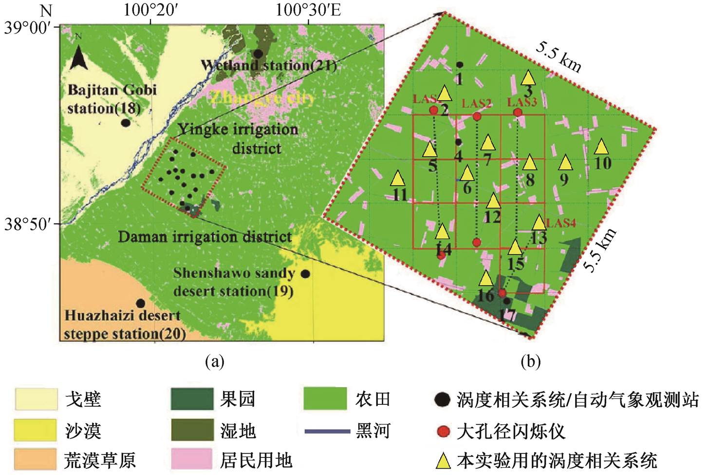
(a) HiWATER计划中21个涡度通量观测塔分布位置; (b)张掖绿洲核心实验区17个涡度通量观测塔位置
图2 研究区概况(改自文献[34,40])
Fig. 2 Study area (modified after Ref. [34,40])
表1 研究区14个涡度相关系统信息
Table 1 Detailed information for 14 eddy covariance systems in the study area
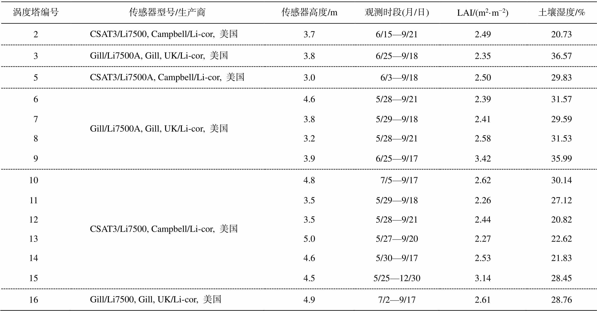
涡度塔编号传感器型号/生产商传感器高度/m观测时段(月/日)LAI/(m2·m−2)土壤湿度/% 2CSAT3/Li7500, Campbell/Li-cor, 美国3.76/15—9/212.4920.73 3Gill/Li7500A, Gill, UK/Li-cor, 美国3.86/25—9/182.3536.57 5CSAT3/Li7500A, Campbell/Li-cor, 美国3.0 6/3—9/182.5029.83 6Gill/Li7500A, Gill, UK/Li-cor, 美国4.65/28—9/212.3931.57 73.85/29—9/182.4129.59 83.25/28—9/212.5831.53 93.96/25—9/173.4235.99 10CSAT3/Li7500, Campbell/Li-cor, 美国4.8 7/5—9/172.6230.14 113.55/29—9/182.2627.12 123.55/28—9/212.4420.82 135.05/27—9/202.2722.62 144.65/30—9/172.5321.83 154.55/25—12/303.1428.45 16Gill/Li7500, Gill, UK/Li-cor, 美国4.97/2—9/172.6128.76
说明: 1)所有的传感器都是开路测量, 相关型号信息引自文献[51]; 2)涡度相关系统的采样频率为 10Hz, 且涡度相关系统数据已按照Liu等[51]的数据处理方法进行质量控制, 处理后的数据为30分钟的平均值; 3)叶面积指数 LAI 和土壤湿度的数据为实验观测期内相应数据的平均值; 4)涡度塔编号与图2(b)中对应; 5)下垫面均为玉米地。
观测期间的叶面积指数 LAI 数据由 LAI-2000 (LI-COR Co., Ltd)实测得到[54]。本研究选取与涡度相关系统和自动气象站观测时间同步的 16 天 LAI实测数据, 分别代表育苗、发芽、抽穗、灌浆和成熟阶段。观测期间研究区气象要素变化如图 3 所示, 太阳辐射、风速、气温和相对湿度的平均值分别为518.70 W/m2, 1.82 m/s, 24.37ºC和46.02%。
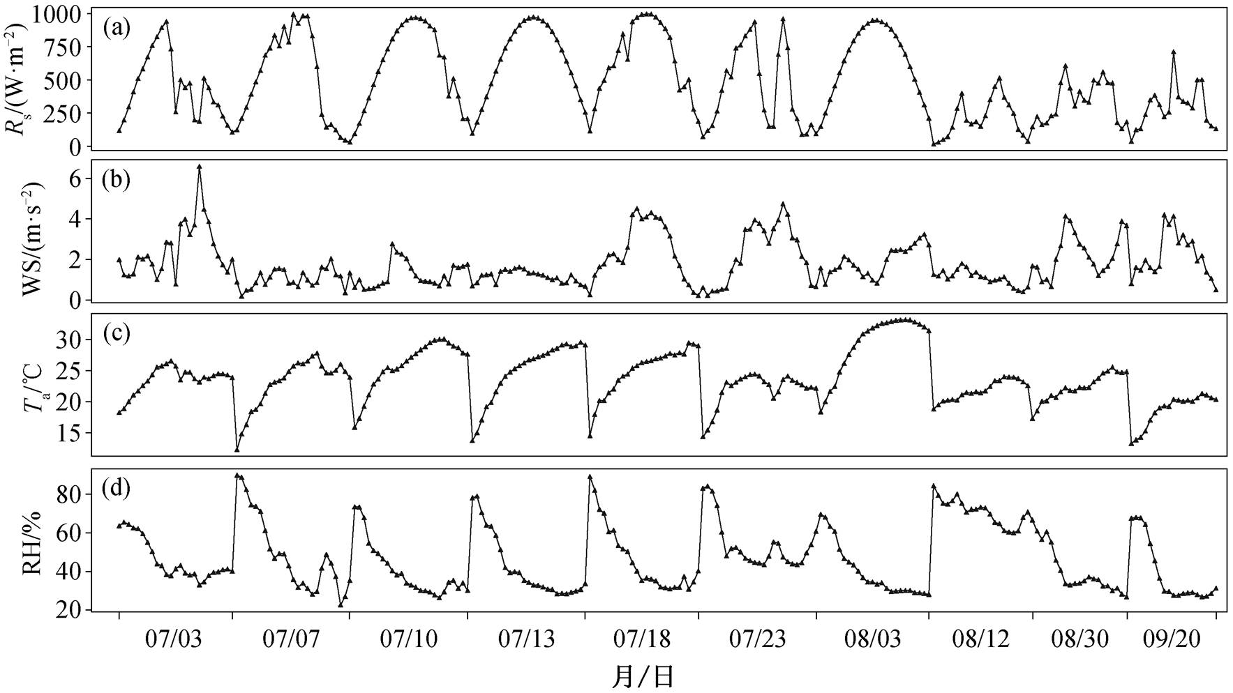
(a)太阳辐射; (b)风速; (c)气温; (d)相对湿度
图3 研究区14个观测站2012年生长季白天(7:00–19:00)气象要素平均概况
Fig. 3 Mean variations in the daytime (7:00–19:00) for meteorological factors for 14 stations during the 2012 growing season
1.2.1 单源Penman-Monteith公式
单源PM公式[12]为
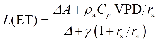 , (1)
, (1)其中, L为潜热蒸发扩散系数; A为可利用的能量(净辐射Rn与土壤热通量G的差值), 由通量塔直接观测得到; VPD为空气的饱和水汽压差, Δ为饱和水汽压对温度曲线的斜率, γ为湿度计算常数, 这3个量均根据Allen等[13]的方法, 基于气象观测数据计算得到; ρa为标准大气压下的空气密度, Cp为空气的比热, rs为表面阻抗。空气动力学阻抗ra根据下式[55–56]计算得到:
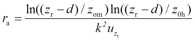 , (2)
, (2)其中, k为冯卡曼常数(k=0.4); Zr 为参考平面高度;  为参考平面风速, d为零平面位移高度, 通常取植被高度的2/3; z0m为动量传输表面粗糙度长度, 为植被冠层高度的0.13倍, z0h是热能的表面粗糙度长度, 为z0m的0.1倍[55]。
单源模型主要包括以下两种。
1)Jarvis-Stewart表面阻抗参数化模型(PM_ JA)。式(1)中的表面阻抗rs可以按照Jarvis-Stewart阻抗模型[27]进行参数化:
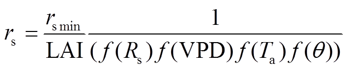 , (3)
, (3)其中, rsmin为最适环境条件下的最小气孔阻抗(如不受环境因子胁迫), f (Rs), f (VPD), f (Ta)和f (θ)采用以下公式[33,57–60]计算:
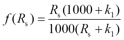 , (4a)
f(VPD)=1−k2VPD, (4b)
 , (4c)
 , (4d)
其中, TL, Top 和 TH 分别为限制气孔活动的最小、最适及最大空气温度, θw 为植被枯萎点, θf 为田间持水力, k1 和 k2 为常量值。各参数取值见表2。
2) KP表面阻抗模型(PM_KP)。在 PM_KP 模型中, rs可用下式表示:
 。 (5)
。 (5)对于经验系数 c1 和 c2, Li 等[33]在本文研究区附近地区(环境状况相似)做过校正, 分别为 0.85 和 1.83 (表2)。r*是与气候变量有关的因子, 计算公式如下:
表2 阻抗参数化的经验参数
Table 2 Empirical parameters used in the surface resistance models
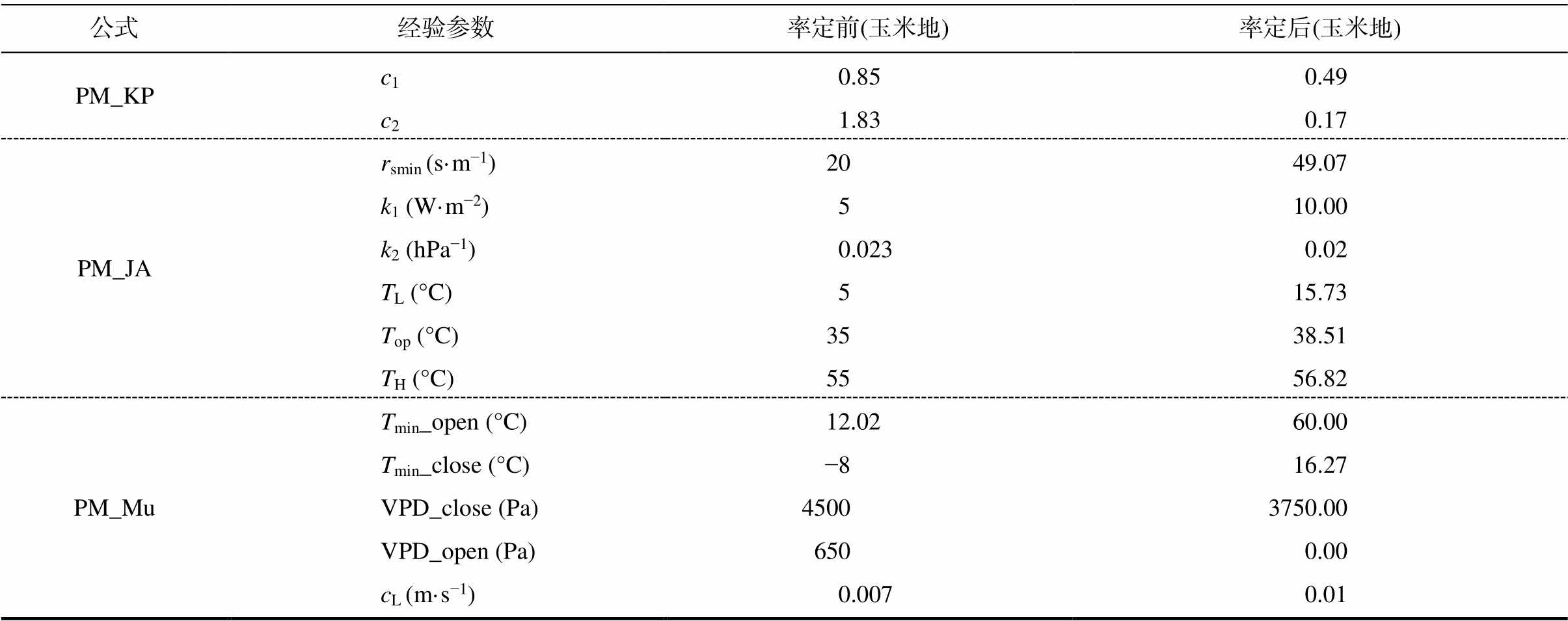
公式经验参数率定前(玉米地)率定后(玉米地) PM_KPc10.850.49 c21.830.17 PM_JArsmin (s·m−1)2049.07 k1 (W·m−2)510.00 k2 (hPa−1)0.0230.02 TL (°C)515.73 Top (°C)3538.51 TH (°C)5556.82 PM_MuTmin_open (°C)12.0260.00 Tmin_close (°C)−816.27 VPD_close (Pa)45003750.00 VPD_open (Pa)6500.00 cL(m·s−1)0.0070.01
说明: 率定前参数取值来源于相应的文献, 如PM_KP和PM_JA方法引自文献[33], PM_Mu方法引自文献[5], 率定后参数值是基于涡度实测潜热通量数据, 使用最小二乘法重新率定后的结果。
 (6)
(6)1.2.2 双源Penman-Monteith公式
Mu 等[5,22]提出, 可以将总蒸散发量(ET)视为冠层蒸腾(Ec)和土壤蒸发(Es)的和, 因此双源 Penman-Monteith公式(PM_Mu)为
 (7)
(7)其中, LEs可根据改进的PM公式[5,21,61]计算:
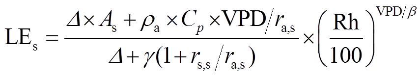 , (8)
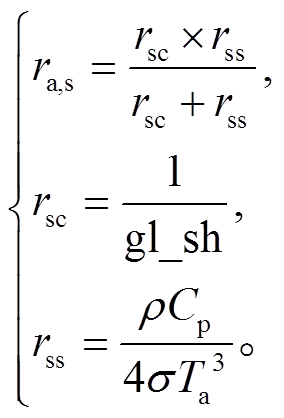
, (8)其中, rs,s为土壤的表面阻抗, ra,s为土壤上方的空气动力学阻抗, 计算公式如下:
 , (9a)
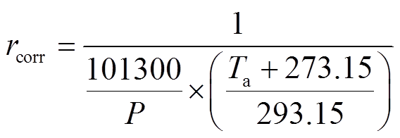 , (9b)
rtot 为未校正的总空气动力学阻抗, 玉米地取值为107 s/m[5]。
 (10)
(10)植被冠层的潜热通量LEc计算公式如下:
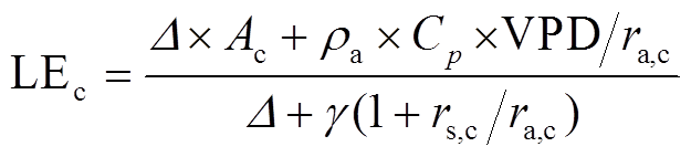 , (11)
ra,c取值与 ra,s 相等, 均由式(10)[21,61]计算得到。
植被冠层的表面阻抗 rs,c 为冠层导度 gc 的倒数:
 , (12)
其中, gc可按照下式计算:
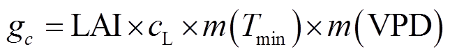 , (13)
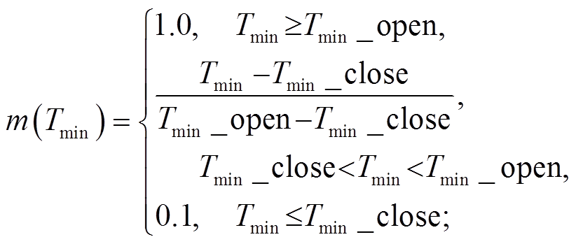 (14a)
(14a)
 (14b)
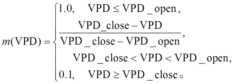
(14b)Tmin_close, Tmin_open, VPD_close 和 VPD_open等参数取值见表2。
1.2.3三温模型
三温模型(3T)由 Qiu[62]于 1996 年基于地表能量平衡提出, 通过引入没有蒸发和蒸腾的干燥参考平面, 避免对难以估算的阻抗进行参数化[63]。三温模型使用参考土壤平面(无蒸发), 并假定参考土壤的空气动力学阻抗与其他土壤表面相同, 从而得到土壤蒸发子模型:
 , (16)
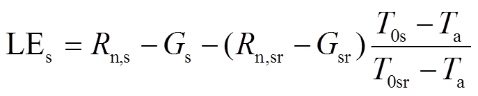
Es 为土壤蒸发分量(mm/s), L 为潜热蒸发系数, Rn,s和 Gs 分别为土壤净辐射分量和土壤热通量(W/m2), Ta 为空气温度(K), Rn,sr, Gsr 与 T0sr 分别为参考平面的净辐射、土壤热通量和表面温度。
同样地, 通过引入参考叶片(无蒸腾), 并假定参考叶片的空气动力学阻抗与周围植被相同, 得到植被蒸腾子模型:
 , (17)
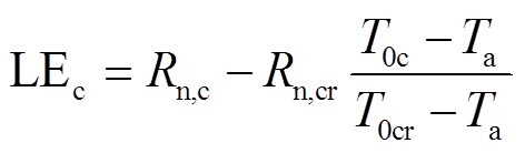
其中, Ec 为植被蒸腾分量(mm/s), Rn,c 为植被净辐射分量, T0c 为冠层表面温度, Rn,cr 和 T0cr 分别是参考平面的净辐射和表面温度。总的潜热通量用式(7)计算得到。本研究以 19 号站点神沙窝沙漠站为参考站点(图 2)。
近年来的研究表明, 三温模型在卫星遥感尺度也可以取得足够好的效果, 是一种相对简单同时足够精确的蒸散发估算方法[41–42,64]。
与涡度实测数据比较, 单源 PM 公式具有比双源 PM 公式更高的蒸散发估算精度, 其中 PM_KP的潜热通量(LE_KP)具有较小的 MAPE (34.08%), 决定系数 R2 为 0.93, RMSE 为 129.22W/m2, PM_JA 的潜热通量(LE_JA)的 MAPE 和 R2 分别为 34.18%和0.79, 均优于双源 PM 模型潜热通量(LE_Mu2007) (MAPE=39.75%, R2=0.34)(图 4), 表明随着蒸散发估算模型结构复杂程度的增加, 模型估算精度有降低的趋势。此外, 虽然三温模型与 PM_Mu 同属于双源蒸散发估算模型, 但由于三温模型中不含与阻抗相关的参数, 避免了由阻抗引起的不确定性, 因此具有较高的精度(MAPE=18.05%, R2=0.85), 优于模型结构更复杂的PM_Mu。
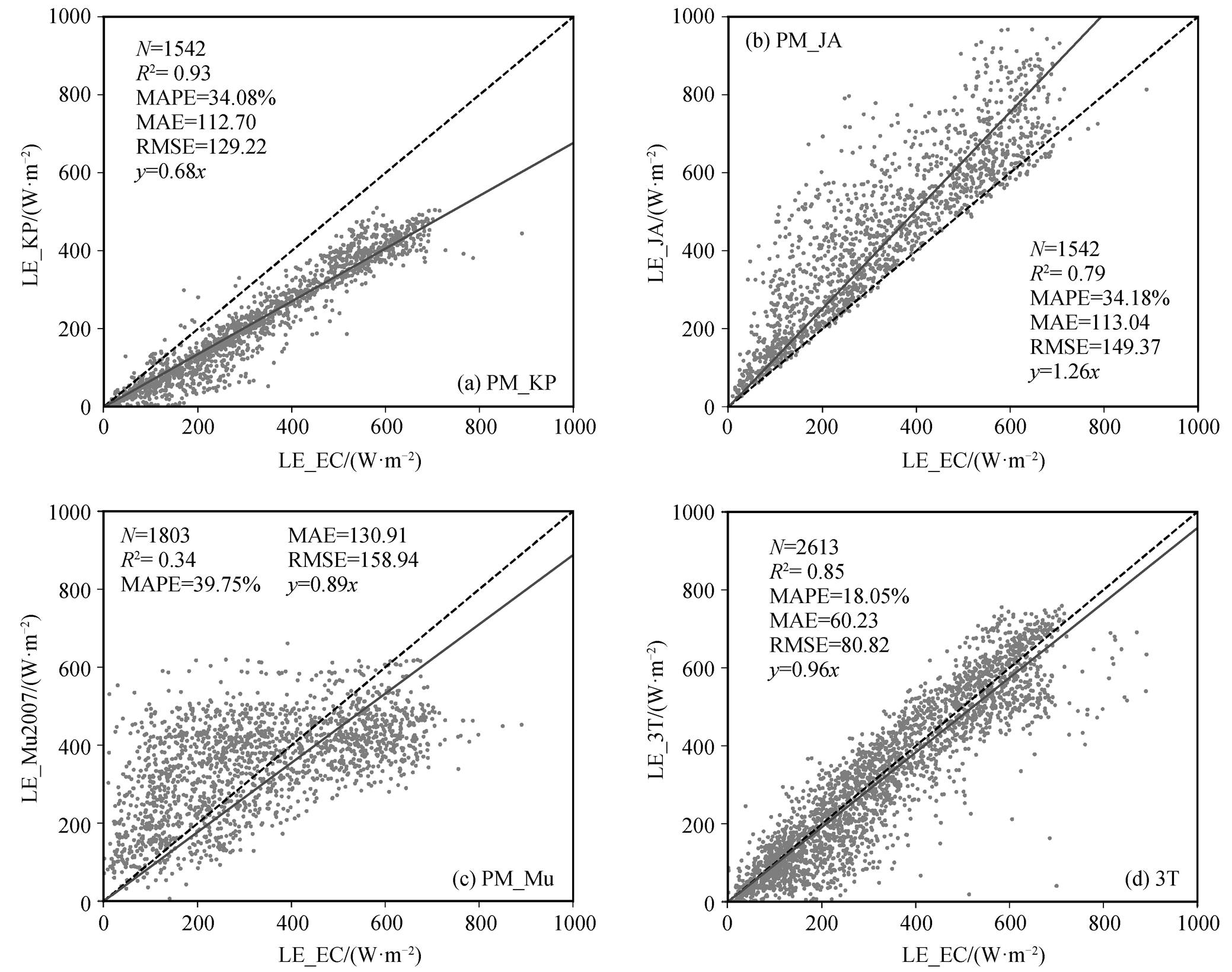
图4 蒸散发估算结果与涡度塔实测数据比较
Fig. 4 Evapotranspiration estimation by Penman-Monteith model and three-temperature model
图 5(a)和(b)分别为根据式(3)和(5)估算得到的PM_KP 和 PM_JA 的冠层表面阻抗 rs_KP 和 rs_JA, 可见由于阻抗参数化过程的不同, 阻抗估算结果会产生较大的差异。即使将阻抗大于 1000s/m 的点作为异常值去除, rs_KP 与 rs_JA 估算值之间的平均值差值仍然可达 231.73s/m, 导致 Penman-Monteith 公式在蒸散发估算中产生差异。例如, 由于 rs_KP 被普遍高估, 导致 LE_KP 呈现明显的低估效应, 而由于 rs_JA 被普遍低估, 导致 LE_JA 呈现明显的高估效应。同样地, 根据式(12)估算得到的 PM_Mu 冠层阻抗分量 rs_veg_Mu2007 也与 rs_KP 和 rs_JA 有较大的差异(图 5(c))。因此, 阻抗参数化过程的不同最终会导致蒸散发估算结果存在较大的差异。
提前使用实测数据对 PM 公式中的经验系数(表2)进行准确率定, 是去除模型结构和参数化差异对蒸散发估算影响的一个可能方案。本研究基于涡度相关系统实测数据, 采用最小二乘法对表 2 中的经验系数进行率定。将观测期内的整个数据集按照1:1 等分成率定数据集和验证数据集。结果表明, 经过提前对经验参数进行率定, 单源 PM 模型的蒸散发估算精度有显著的提升, 率定后 PM_KP 的潜热通量LE_KP_cal 的低估效应得到改善, 无偏回归线的斜率为 0.98 (图 6(a)), 散点均匀地分布在 1:1 线两侧, MAPE 仅为 12.42%, RMSE 为 59.73W/m2。同样, 率定后 PM_JA 的潜热通量 LE_JA_cal 结果不再呈现高估效应, 无偏回归线的斜率为 0.97, 接近1, MAPE 和 RMSE 分别降低到 14.38%和 60.73 W/m2(图 6(b))。表 2 中经验参数的率定前取值来自 Li 等[33]在黑河地区的研究结果, 但在本研究中, 率定后的经验参数值与原值有差别, 表明即使是气候、地理环境条件都相似的地区, 仍然需要用实测数据重新率定经验系数, 这些经验系数过分依赖率定数据集, 使得 PM 公式在缺乏气象观测资料的地区难以应用, 而不含经验系数的三温模型可以达到较好的蒸散发估算效果。此外, 率定后 PM_KP 的蒸散发估算结果仍然优于 PM_JA (图 4 和 6), 这同样表明对于单源 PM 公式而言, 模型含有的经验系数越少, 阻抗参数化模型越简单, 引起的蒸散发估算误差就越小。这可能是因为当观测数据量有限时, 模型越简单, 越容易获得更符合观测数据集的率定结果。
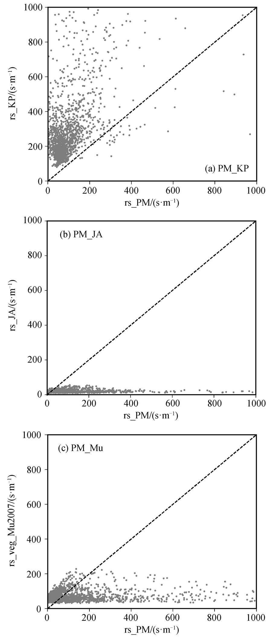
图5 冠层表面阻抗模拟结果与Penman-Monteith公式逆推阻抗比较
Fig. 5 Canopy resistance estimated by resistance model and the inverse of the PM equation
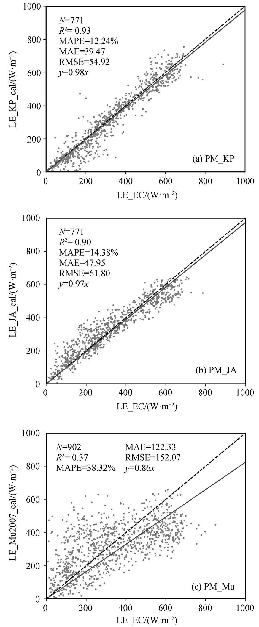
图6 Penman-Monteith公式率定参数后蒸散发估算结果与涡度塔实测数据比较
Fig. 6 Evapotranspiration estimation by Penman-Monteith model and three-temperature model
相比之下, 率定经验系数后, 双源 PM 公式的蒸散发估算精度只有轻微的提升, 率定后的蒸散发估算结果 MAPE 为 38.96%, 略低于参数率定前的MAPE (39.75%), 精度仅提升 0.79%, 率定后的潜热通量 LE_Mu2007_cal 仍然呈现低估的趋势(图 6(c)), 表明与单源 PM 公式中较简单的阻抗参数化过程相比, 更复杂的双源阻抗参数化结构可能会导致更大的误差。
本文基于黑河高密度通量观测数据, 研究模型结构和参数化差异对蒸散发估算结果的影响, 主要结论如下。
1)随着模型结构复杂程度增加, 蒸散发估算精度有降低的趋势。单源 PM 公式具有比模型结构更复杂的双源 PM 公式更高的蒸散发估算精度, 不含阻抗的双源三温模型具有比双源 PM 公式更高的蒸散发估算精度。
2)随着阻抗参数化复杂程度增加, 蒸散发估算精度有降低的趋势。只含两个经验系数的 PM_KP公式具有比含 6 个经验系数的 PM_JA 略高的估算精度, 且显著优于含 5 个经验系数、阻抗参数化更复杂的双源结构PM_Mu模型。
3)使用实测数据对 PM 公式中的经验系数提前进行率定, 可以在一定程度上去除模型结构和阻抗参数化对蒸散发估算结果的影响。率定后, 模型结构相对较简单的单源 PM 公式蒸散发估算精度均有显著的提升(PM_KP 和 PM_JA 的 MAPE 分别降低22%和 20%), 但双源 PM_Mu 由于模型结构和阻抗参数化过于复杂, 即使采用观测数据率定后, 蒸散发估算精度也无明显的改善(MAPE 仅减小 0.8%)。
综上所述, 模型结构及其参数化过程对蒸散发估算影响较大, 在未来的研究中应予以重视。
参考文献
[1] Yan C, Qiu G. The three-temperature model to est-imate evapotranspiration and its partitioning at mul-tiple scales: a review. Transactions of the ASABE, 2016, 59(2): 661–670
[2] Kite G, Droogers P. Comparing evapotranspiration es-timates from satellites, hydrological models and field data. Journal of Hydrology, 2000, 229(1/2): 3–18
[3] 赵玲玲, 夏军, 许崇育, 等. 水文循环模拟中蒸散发估算方法综述. 地理学报, 2013, 68(1): 127–136
[4] Zhao W L, Gentine P, Reichstein M, et al. Physics-constrained machine learning of evapotranspiration. Geophysical Research Letters, 2019, 46(24): 14496–14507
[5] Mu Q, Heinsch F A, Zhao M, et al. Development of a global evapotranspiration algorithm based on MODIS and global meteorology data. Remote Sensing of En-vironment, 2007, 111(4): 519–536
[6] Jung M, Reichstein M, Ciais P, et al. Recent decline in the global land evapotranspiration trend due to limited moisture supply. Nature, 2010, 467: 951–954
[7] 李晓媛, 于德永. 蒸散发估算方法及其驱动力研究进展. 干旱区研究, 2020, 37(1): 26–36
[8] Chen Y, Xia J, Liang S, et al. Comparison of satellite-based evapotranspiration models over terrestrial eco-systems in China. Remote Sensing of Environment, 2014, 140: 279–293
[9] 冯景泽, 王忠静. 遥感蒸散发模型研究进展综述. 水利学报, 2012, 43(8): 914–925
[10] Ershadi A, McCabe M, Evans J, et al. Impact of model structure and parameterization on Penman–Monteith type evaporation models. Journal of Hydro-logy, 2015, 525: 521–535
[11] Penman H L. Natural evaporation from open water, bare soil and grass. Proceedings of the Royal Society of London. Series A. Mathematical and Physical Sciences, 1948, 193: 120–145
[12] Monteith J L. Evaporation and environment // 19th Symposia of the Society for Experimental Biology. Cambridge: Cambridge University Press, 1965: 205–234
[13] Allen R G, Pereira L S, Raes D, et al. Crop evapo-transpiration — guidelines for computing crop water requirements — FAO irrigation and drainage paper 56. Rome: FAO, 1998
[14] Shuttleworth W J, Wallace J. Evaporation from sparse crops — an energy combination theory. Quarterly Journal of the Royal Meteorological Society, 1985, 111: 839–855
[15] Rana G, Katerji N. A measurement based sensitivity analysis of the Penman-Monteith actual evapotranspi-ration model for crops of different height and in con-trasting water status. Theoretical and Applied Clima-tology, 1998, 60(1/2/3/4): 141–149
[16] Norman J M, Kustas W P, Humes K S. Source app-roach for estimating soil and vegetation energy fluxes in observations of directional radiometric surface tem-perature. Agricultural and Forest Meteorology, 1995, 77(3/4): 263–293
[17] Boulet G, Mougenot B, Lhomme J P, et al. The SPARSE model for the prediction of water stress and evapotranspiration components from thermal infra-red data and its evaluation over irrigated and rainfed wheat. Hydrology and Earth System Sciences Discus-sions, 2015(19): 4653–4672
[18] Li X, Gentine P, Lin C, et al. A simple and objective method to partition evapotranspiration into transpi-ration and evaporation at eddy-covariance sites. Agri-cultural and Forest Meteorology, 2019, 265: 171–182
[19] Cleugh H A, Leuning R, Mu Q, et al. Regional evapo-ration estimates from flux tower and MODIS satellite data. Remote Sensing of Environment, 2007, 106(3): 285–304
[20] Leuning R, Zhang Y Q, Rajaud A, et al. A simple surface conductance model to estimate regional evapo-ration using MODIS leaf area index and the Penman-Monteith equation. Water Resources Research, 2008, 44(10): W10419
[21] Zhang K, Kimball J S, Nemani R R, et al. A conti-nuous satellite-derived global record of land surface evapotranspiration from 1983 to 2006. Water Resour-ces Research, 2010, 46(9): W09522
[22] Mu Q, Zhao M, Running S W. Improvements to a MODIS global terrestrial evapotranspiration algorithm. Remote Sensing of Environment, 2011, 115(8): 1781–1800
[23] Yao Y, Liang S, Li X, et al. A satellite-based hybrid algorithm to determine the Priestley–Taylor parameter for global terrestrial latent heat flux estimation across multiple biomes. Remote Sensing of Environment, 2015, 165: 216–233
[24] Peng L, Zeng Z, Wei Z, et al. Determinants of the ratio of actual to potential evapotranspiration. Global change biology, 2019, 25(4): 1326–1343
[25] 杨雨亭, 尚松浩. 双源蒸散发模型估算潜在蒸散发量的对比. 农业工程学报, 2012, 28(24): 85–91
[26] 高冠龙, 张小由, 鱼腾飞, 等. Shuttleworth-Wallace 双源蒸散发模型阻力参数的确定. 冰川冻土, 2016, 38(1): 170–177
[27] Jarvis P. The interpretation of the variations in leaf water potential and stomatal conductance found in canopies in the field. Philosophical Transactions of the Royal Society of London, Series B, Biological Sciences, 1976, 273: 593–610
[28] Tan Z H, Zhao J F, Wang G Z, et al. Surface conductance for evapotranspiration of tropical forests: Calculations, variations, and controls. Agricultural and Forest Meteorology, 2019, 275: 317–328
[29] Katerji N, Rana G, Fahed S. Parameterizing canopy resistance using mechanistic and semi-empirical esti-mates of hourly evapotranspiration: critical evaluation for irrigated crops in the Mediterranean. Hydrological Processes, 2011, 25(1): 117–129
[30] Xu J, Liu X, Yang S, et al. Modeling rice evapo-transpiration under water-saving irrigation by cali-brating canopy resistance model parameters in the Penman-Monteith equation. Agricultural Water Manage-ment, 2017, 182: 55–66
[31] Lehmann P, Merlin O, Gentine P, et al. Soil texture effects on surface resistance to bare-soil evaporation. Geophysical Research Letters, 2018, 45(19): 10398–10405
[32] Leuning R, Zhang Y, Rajaud A, et al. A simple surface conductance model to estimate regional evaporation using MODIS leaf area index and the Penman-Monteith equation. Water Resources Research, 2008, 44(10): W10419
[33] Li S, Zhang L, Kang S, et al. Comparison of several surface resistance models for estimating crop evapo-transpiration over the entire growing season in arid regions. Agricultural and Forest Meteorology, 2015, 208: 1–15
[34] Li Y, Kustas W P, Huang C, et al. Evaluation of soil resistance formulations for estimates of sensible heat flux in a desert vineyard. Agricultural and forest me-teorology, 2018, 260: 255–261
[35] Long D, Longuevergne L, Scanlon B R. Uncertainty in evapotranspiration from land surface modeling, re-mote sensing, and GRACE satellites. Water Resour-ces Research, 2014, 50(2): 1131–1151
[36] Ershadi A, McCabe M F, Evans J P, et al. Impact of model structure and parameterization on Penman–Monteith type evaporation models. Journal of Hydro-logy, 2015, 525: 521–535
[37] Zhang K, Kimball J S, Running S W. A review of remote sensing based actual evapotranspiration esti-mation. Wiley Interdisciplinary Reviews: Water, 2016, 3(6): 834–853
[38] Yao Y, Liang S, Yu J, et al. Differences in estima- ting terrestrial water flux from three satellite-based Priestley-Taylor algorithms. International Journal of Applied Earth Observation and Geoinformation, 2017, 56: 1–12
[39] 王宁, 贾立, 李占胜, 等. 非参数化蒸散发估算方法在黑河流域的适用性分析. 高原气象, 2016, 35 (1): 118–128
[40] Qiu G Y, Shi P, Wang L. Theoretical analysis of a remotely measurable soil evaporation transfer coeffi-cient. Remote Sensing of Environment, 2006, 101(3): 390–398
[41] Xiong Y J, Zhao S H, Tian F, et al. An evapotranspi-ration product for arid regions based on the three-temperature model and thermal remote sensing. Jour-nal of Hydrology, 2015, 530: 392–404
[42] Wang Y Q, Xiong Y J, Qiu G Y, et al. Is scale really a challenge in evapotranspiration estimation? A multi-scale study in the Heihe oasis using thermal remote sensing and the three-temperature model. Agricultural and Forest Meteorology, 2016, 230/231: 128–141
[43] Priestley C H B, Taylor R. On the assessment of surface heat flux and evaporation using large-scale parameters. Monthly Weather Review, 1972, 100(2): 81–92
[44] Ma N, Szilagyi J, Zhang Y, et al. Complementary-relationship-based modeling of terrestrial evapotran-spiration across China during 1982–2012: validations and spatiotemporal analyses. Journal of Geophysical Research: Atmospheres, 2019, 124(8): 4326–4351
[45] 韩松俊, 张宝忠. 基于 Penman 方法和互补原理的蒸散发研究历程与展望. 水利学报, 2018, 49(9): 1158–1168
[46] Long D, Singh V P. A two-source trapezoid model for evapotranspiration (TTME) from satellite imagery. Re-mote Sensing of Environment, 2012, 121: 370–388
[47] 刘元波, 张珂. 最大熵增地表蒸散模型: 原理及应用综述. 地球科学进展, 2019, 34(6): 596–605
[48] Ershadi A, McCabe M, Evans J P, et al. Multi-site evaluation of terrestrial evaporation models using FLUXNET data. Agricultural and Forest Meteorology, 2014, 187: 46–61
[49] Zhou X, Bi S, Yang Y, et al. Comparison of ET estimations by the three-temperature model, SEBAL model and eddy covariance observations. Journal of Hydrology, 2014, 519: 769–776
[50] 蒙吉军, 汪疆玮, 王雅, 等. 基于绿洲灌区尺度的生态需水及水资源配置效率研究——黑河中游案例. 北京大学学报(自然科学版), 2018, 54(1): 171–180
[51] Liu S, Xu Z, Song L, et al. Upscaling evapotranspira-tion measurements from multi-site to the satellite pixel scale over heterogeneous land surfaces. Agri-cultural and Forest Meteorology, 2016, 230: 97–113
[52] Twine T E, Kustas W, Norman J, et al. Correcting eddy-covariance flux underestimates over a grassland. Agricultural and Forest Meteorology, 2000, 103(3): 279–300
[53] Xu Z, Liu S, Li X, et al. Intercomparison of surface energy flux measurement systems used during the HiWATER-MUSOEXE. Journal of Geophysical Re-search: Atmospheres, 2013, 118(23): 13140–13157
[54] Qu Y, Zhu Y, Han W, et al. Crop leaf area index observations with a wireless sensor network and its potential for validating remote sensing products. IEEE Journal of Selected Topics in Applied Earth Observations and Remote Sensing, 2013, 7(2): 431–444
[55] Brutsaert W, Stricker H. An advection-aridity approa-ch to estimate actual regional evapotranspiration. Water Resources Research, 1979, 15(2): 443–450
[56] Irmak S, Mutiibwa D, Irmak A, et al. On the scaling up leaf stomatal resistance to canopy resistance using photosynthetic photon flux density. Agricultural and Forest Meteorology, 2008, 148(6/7): 1034–1044
[57] Li S, Kang S, Zhang L, et al. Quantifying the com-bined effects of climatic, crop and soil factors on surface resistance in a maize field. Journal of Hydro-logy, 2013, 489: 124–134
[58] Bai Y, Li X, Liu S, et al. Modelling diurnal and seasonal hysteresis phenomena of canopy conductance in an oasis forest ecosystem. Agricultural and Forest Meteorology, 2017, 246: 98–110
[59] Bai Y, Li X, Zhou S, et al. Quantifying plant trans-piration and canopy conductance using eddy flux data: an underlying water use efficiency method. Agricultu-ral and Forest Meteorology, 2019, 271: 375–384
[60] Hu G, Jia L. Monitoring of evapotranspiration in a semi-arid inland river basin by combining microwave and optical remote sensing observations. Remote Sensing, 2015, 7(3): 3056–3087
[61] Zhang K, Kimball J S, Mu Q, et al. Satellite based analysis of northern ET trends and associated changes in the regional water balance from 1983 to 2005. Journal of Hydrology, 2009, 379(1): 92–110
[62] Qiu G Y. Estimation of plant transpiration by imita-tion leaf temperature II. application of imitation leaf temperature for detection of crop water stress. Tran-sactions of the Japanese Society of Irrigation, Drai-nage and Reclamation Engineering, 1996, 64(5): 767–773
[63] Paw U K T, Daughtry C S T. A new method for the estimation of diffusive resistance of leaves. Agricul-tural and Forest Meteorology, 1984, 33(2): 141–155
[64] Xiong Y J, Qiu G Y. Estimation of evapotranspiration using remotely sensed land surface temperature and the revised three-temperature model. International Journal of Remote Sensing, 2011, 32(20): 5853–5874
Impact of Model Structure and Parameterization Differences on Evapotranspiration Estimation
Abstract Based on the HiWATER high-density eddy covariance (EC) tower observations in Heihe Oasis in 2012, the impact of model structure differences (comparison between one-source Penman-Monteith / PM equation and two-source PM equation, or comparison between two-source PM equation and two-source three-temperature model) and parameterization differences on the evapotranspiration estimation were evaluated. The results show that, 1) compared with the two-source PM equation with a relatively complex model structure, the mean absolute percent error (MAPE) estimated by the one-source PM equation is 34%, which is more accurate than that by the two-source PM equation (40%); 2) for two kinds of two-source model with significant differences in model structure, the three-temperature model without resistance parameters has higher estimation accuracy than the PM-based equation with resistance parameters. The former has a MAPE of 18% (R2=0.85), while the PM-based equation has that of 40% (R2=0.34); 3) two one-source and one two-source resistance parameterization methods lead to different evapotranspiration estimation accuracy for the PM-based equation, with a MAPE difference of up to 6%; 4) using prior knowledge / dataset to calibrate resistance parameterization can significantly improve the estimation accuracy of one-source PM equation (MAPE can be reduced by 22%), but as model structure and parameterization complexity increase, two-source PM equation hasn’t been improved significantly after resistance parameterization calibration (MAPE is only reduced by 0.8%).
Key words evapotranspiration; Penman-Monteith; resistance; three-temperature model; HiWATER; Heihe
doi: 10.13209/j.0479-8023.2020.119
收稿日期: 2020–01–14;
修回日期: 2020–03–15
深圳市知识创新计划(JCYJ20180504165440088)和国家自然科学基金(41671416)资助